-
Notifications
You must be signed in to change notification settings - Fork 147
Dec 29, 2020
- Introduction
- 1 Regularized Linear Regression
- 2 Bias-variance
-
3 Polynomial regression
- 3.1 Learning Polynomial Regression
- 3.2 Optional (ungraded) exercise: Adjusting the regularization parameter
- 3.3 Selecting
 using a cross validation
set
 - 3.4 Optional (ungraded) exercise: Computing test set error
- 3.5 Optional (ungraded) exercise: Plotting learning curves with randomly selected examples
- Submission and Grading
This programming exercise instruction was originally developed and written by Prof. Andrew Ng as part of his machine learning course on Coursera platform. I have adapted the instruction for R language, so that its users, including myself, could also take and benefit from the course.
In this exercise, you will implement regularized linear regression and
use it to study models with different bias-variance properties. Before
starting on the programming exercise, we strongly recommend watching the
video lectures and completing the review questions for the associated
topics. To get started with the exercise, you will need to download the
starter code and unzip its contents to the directory where you wish to
complete the exercise. If needed, use the setwd() function in R to
change to this directory before starting this exercise.
Files included in this exercise
-
ex5.R- R script that steps you through the exercise -
ex5data1.Rda- Dataset -
submit.R- Submission script that sends your solutions to our servers -
featureNormalize.R- Feature normalization function -
plotFit.R- Plot a polynomial fit -
trainLinearReg.R- Trains linear regression using your cost function - [⋆]
linearRegCostFunction.R- Regularized linear regression cost function - [⋆]
learningCurve.R- Generates a learning curve - [⋆]
polyFeatures.R- Maps data into polynomial feature space - [⋆]
validationCurve.R- Generates a cross validation curve
⋆ indicates files you will need to complete
Throughout the exercise, you will be using the script ex5.R. These
scripts set up the dataset for the problems and make calls to functions
that you will write. You are only required to modify functions in other
files, by following the instructions in this assignment.
The exercises in this course use R, a high-level programming language
well-suited for numerical computations. If you do not have R installed,
please download a Windows installer from
R-project website.
R-Studio is a free and
open-source R integrated development environment (IDE) making R script
development a bit easier when compared to the R’s own basic GUI. You may
start from the .Rproj (a R-Studio project file) in each exercise
directory. At the R command line, typing help followed by a function
name displays documentation for that function. For example,
help('plot') or simply ?plot will bring up help information for
plotting. Further documentation for R functions can be found at the R
documentation pages.
In the first half of the exercise, you will implement regularized linear
regression to predict the amount of water flowing out of a dam using the
change of water level in a reservoir. In the next half, you will go
through some diagnostics of debugging learning algorithms and examine
the effects of bias v.s. variance. The provided script, ex5.R, will
help you step through this exercise.
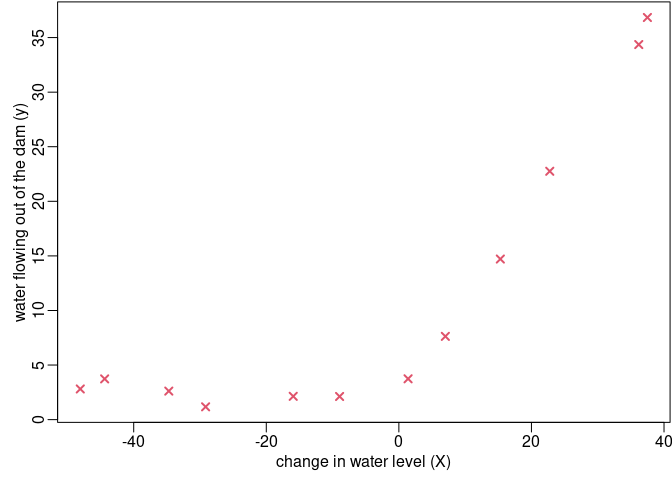
We will begin by visualizing the dataset containing historical records
on the change in the water level,  , and the
amount of water flowing out of the dam,
  . This
dataset is divided into three parts:
- A training set that your model will learn on:
X, y - A cross validation set for determining the regularization
parameter:
Xval, yval - A test set for evaluating performance. These are “unseen”
examples which your model did not see during training:
Xtest, ytest
The next step of ex5.R will plot the training data (Figure 1). In the
following parts, you will implement linear regression and use that to
fit a straight line to the data and plot learning curves. Following
that, you will implement polynomial regression to find a better fit to
the data.

Figure 1: Data
Recall that regularized linear regression has the following cost function:

where  is a regularization parameter which
controls the degree of regularization (thus, help preventing
overfitting). The regularization term puts a penalty on the overal cost
 . As the magnitudes of the model parameters
 increase, the penalty increases as well. Note
that you should not regularize the
  term. (In R,
the
  term is represented as
 theta[1] since
indexing in R starts from 1). You should now complete the code in the
file linearRegCostFunction.R. Your task is to write a function to
calculate the regularized linear regression cost function. If possible,
try to vectorize your code and avoid writing loops. When you are
finished, the next part of ex5.R will run your cost function using
theta initialized at c(1,1). You should expect to see an output of
303.993.
You should now submit your solutions.
Correspondingly, the partial derivative of regularized linear
regression’s cost for  is defined as

In linearRegCostFunction.R, add code to calculate the gradient,
returning it in the variable grad. When you are finished, the next part
of ex5.R will run your gradient function using theta initialized at
c(1,1). You should expect to see a gradient of c(-15.30, 598.250).
You should now submit your solutions.
Once your cost function and gradient are working correctly, the next
part of ex5.R will run the code in trainLinearReg.R to compute the
optimal values of  . This training function uses
optim to optimize the cost function. In this part, we set
regularization parameter  to zero. Because our
current implementation of linear regression is trying to fit a
2-dimensional
  , regularization will not be
incredibly helpful for a
  of such low dimension.
In the later parts of the exercise, you will be using polynomial
regression with regularization. Finally, the
 ex5.R script should also
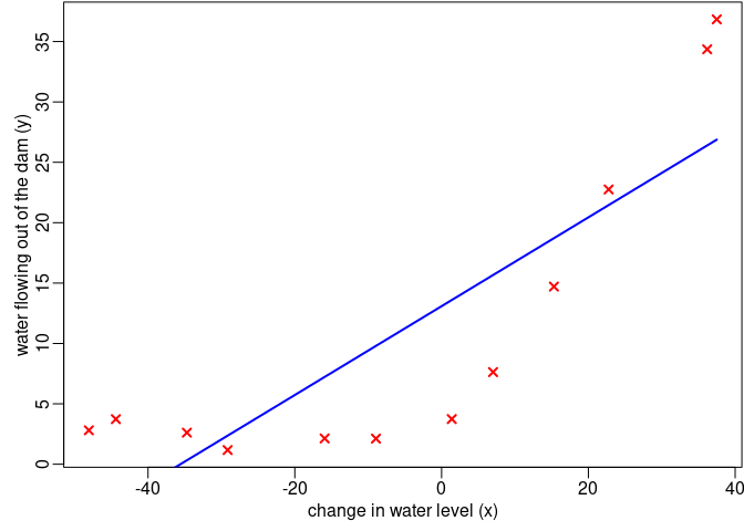
plot the best fit line, resulting in an image similar to Figure 2. The
best fit line tells us that the model is not a good fit to the data
because the data has a non-linear pattern. While visualizing the best
fit as shown is one possible way to debug your learning algorithm, it is
not always easy to visualize the data and model. In the next section,
you will implement a function to generate learning curves that can help
you debug your learning algorithm even if it is not easy to visualize
the data.

Figure 2: Linear Fit
An important concept in machine learning is the bias-variance tradeoff. Models with high bias are not complex enough for the data and tend to underfit, while models with high variance overfit to the training data.
In this part of the exercise, you will plot training and test errors on a learning curve to diagnose bias-variance problems.
You will now implement code to generate the learning curves that will be
useful in debugging learning algorithms. Recall that a learning curve
plots training and cross validation error as a function of training set
size. Your job is to fill in learningCurve.R so that it returns a
vector of errors for the training set and cross validation set. To plot
the learning curve, we need a training and cross validation set error
for different training set sizes. To obtain different training set
sizes, you should use different subsets of the original training set
 . Specifically, for a training set size of i, you
should use the first i examples (i.e.,
 X[1:i,] and y[1:i]). You can
use the trainLinearReg function to find the  parameters. Note that the
 lambda is passed as a parameter to the
learningCurve function. After learning the  parameters, you should compute the error on the training and cross
validation sets. Recall that the training error for a dataset is defined
as

In particular, note that the training error does not include the
regularization term. One way to compute the training error is to use
your existing cost function and set  to 0 only
when using it to compute the training error and cross validation error.
When you are computing the training set error, make sure you compute it
on the training subset (i.e.,
 X[1:n,] and y[1:n]) (instead of the
entire training set). However, for the cross validation error, you
should compute it over the entire cross validation set. You should store
the computed errors in the vectors error train and error val. When you
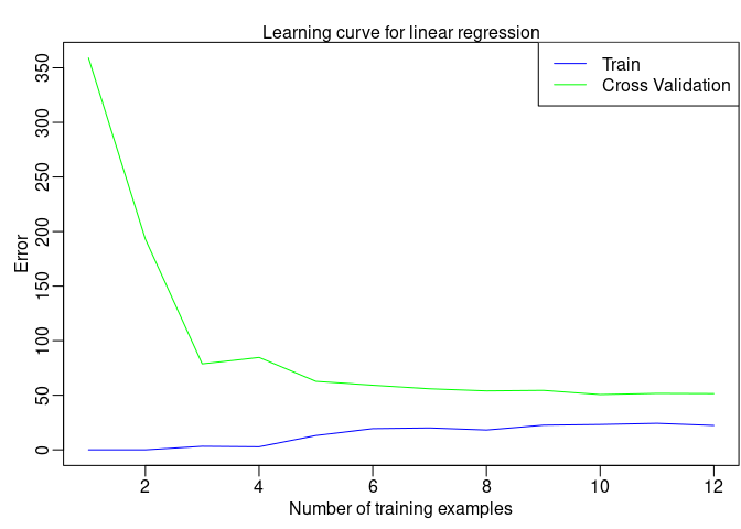
are finished, ex5.R wil print the learning curves and produce a plot
similar to Figure 3.
You should now submit your solutions.
In Figure 3, you can observe that both the train error and cross validation error are high when the number of training examples is increased. This reflects a high bias problem in the model – the linear regression model is too simple and is unable to fit our dataset well. In the next section, you will implement polynomial regression to fit a better model for this dataset.

Figure 3: Linear regression learning curve
The problem with our linear model was that it was too simple for the data and resulted in underfitting (high bias). In this part of the exercise, you will address this problem by adding more features. For use polynomial regression, our hypothesis has the form:

Notice that by defining  , we obtain a linear
regression model where the features are the various powers of the
original value (waterLevel). Now, you will add more features using the
higher powers of the existing feature
  in the
dataset. Your task in this part is to complete the code in
polyFeatures.R so that the function maps the original training set X
of size  into its higher powers. Specifically,
when a training set
 X of size  is passed into
the function, the function should return a
  matrix
X_poly, where column 1 holds the original values of X, column 2
holds the values of X^2, column 3 holds the values of X^3, and so
on. Note that you don’t have to account for the zero-eth power in this
function. Now you have a function that will map features to a higher
dimension, and Part 6 of ex5.R will apply it to the training set, the
test set, and the cross validation set (which you haven’t used yet).
You should now submit your solutions.
After you have completed polyFeatures.R, the ex5.R script will
proceed to train polynomial regression using your linear regression cost
function. Keep in mind that even though we have polynomial terms in our
feature vector, we are still solving a linear regression optimization
problem. The polynomial terms have simply turned into features that we
can use for linear regression. We are using the same cost function and
gradient that you wrote for the earlier part of this exercise. For this
part of the exercise, you will be using a polynomial of degree 8. It
turns out that if we run the training directly on the projected data,
will not work well as the features would be badly scaled (e.g., an
example with  will now have a feature
 ). Therefore, you will need to use feature
normalization. Before learning the parameters
  for
the polynomial regression,
 ex5.R will first call featureNormalize
and normalize the features of the training set, storing the mu,
sigma parameters separately. We have already implemented this function
for you and it is the same function from the first exercise. After
learning the parameters  , you should see two plots
(Figure 4,5) generated for polynomial regression with
 . From Figure 4, you should see that the
polynomial fit is able to follow the datapoints very well - thus,
obtaining a low training error. However, the polynomial fit is very
complex and even drops off at the extremes. This is an indicator that
the polynomial regression model is overfitting the training data and
will not generalize well. To better understand the problems with the
unregularized (
 ) model, you can see that the
learning curve (Figure 5) shows the same effect where the low training
error is low, but the cross validation error is high. There is a gap
between the training and cross validation errors, indicating a high
variance problem.
](5/tmp_files/figure-gfm/unnamed-chunk-4-1.png)
Figure 4: Polynomial fit, 
](5/tmp_files/figure-gfm/unnamed-chunk-5-1.png)
Figure 5: Polynomial learning curve, 
One way to combat the overfitting (high-variance) problem is to add
regularization to the model. In the next section, you will get to try
different  parameters to see how regularization
can lead to a better model.
In this section, you will get to observe how the regularization
parameter affects the bias-variance of regularized polynomial
regression. You should now modify the lambda parameter in the ex5.R
and try  . For each of these values, the script
should generate a polynomial fit to the data and also a learning curve.
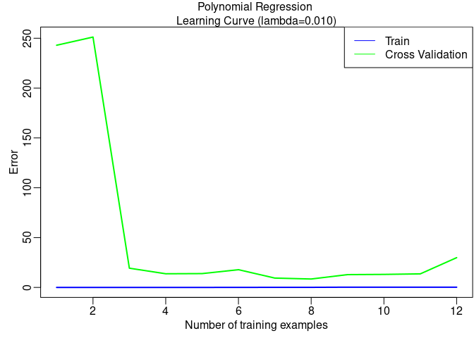
For
  , you should see a polynomial fit that
follows the data trend well (Figure 6) and a learning curve (Figure 7)
showing that both the cross validation and training error converge to a
relatively low value. This shows the
  regularized
polynomial regression model does not have the high bias or high-variance
problems. In effect, it achieves a good trade-off between bias and
variance. For
  , you should see a polynomial fit
(Figure 8) that does not follow the data well. In this case, there is
too much regularization and the model is unable to fit the training
data.
You do not need to submit any solutions for this optional (ungraded) exercise.
](5/tmp_files/figure-gfm/unnamed-chunk-6-1.png)
Figure 6: Polynomial fit, 
](5/tmp_files/figure-gfm/unnamed-chunk-7-1.png)
Figure 7: Polynomial learning curve, 
](5/tmp_files/figure-gfm/unnamed-chunk-8-1.png)
Figure 8: Polynomial fit, 
From the previous parts of the exercise, you observed that the value of
 can significantly affect the results of
regularized polynomial regression on the training and cross validation
set. In particular, a model without regularization
(
 ) fits the training set well, but does not
generalize. Conversely, a model with too much regularization
(
 = 100) does not fit the training set and
testing set well. A good choice of
  (e.g.,
 ) can provide a good fit to the data. In this
section, you will implement an automated method to select the
 parameter. Concretely, you will use a cross
validation set to evaluate how good each
  value
is. After selecting the best
  value using the
cross validation set, we can then evaluate the model on the test set to
estimate how well the model will perform on actual unseen data. Your
task is to complete the code in
 validationCurve.R. Specifically, you
should should use the trainLinearReg function to train the model using
different values of  and compute the training
error and cross validation error. You should try
  in the following range:
  .
.
 using a cross validation set](5/tmp_files/figure-gfm/unnamed-chunk-9-1.png)
Figure 9: Selecting  using a cross validation set
After you have completed the code, the next part of ex5.R will run
your function can plot a cross validation curve of error v.s.
 that allows you select which
 parameter to use. You should see a plot similar
to Figure 9. In this figure, we can see that the best value of
 is around 3. Due to randomness in the training
and validation splits of the dataset, the cross validation error can
sometimes be lower than the training error.
You should now submit your solutions.
In the previous part of the exercise, you implemented code to compute
the cross validation error for various values of the regularization
parameter λ. However, to get a better indication of the model’s
performance in the real world, it is important to evaluate the “final”
model on a test set that was not used in any part of training (that is,
it was neither used to select the  parameters,
nor to learn the model parameters
  ). For this
optional (ungraded) exercise, you should compute the test error using
the best value of
  you found. In our cross
validation, we obtained a test error of
  for
for
 .
.
You do not need to submit any solutions for this optional (ungraded) exercise.
In practice, especially for small training sets, when you plot learning
curves to debug your algorithms, it is often helpful to average across
multiple sets of randomly selected examples to determine the training
error and cross validation error. Concretely, to determine the training
error and cross validation error for i examples, you should first
randomly select i examples from the training set and i examples from the
cross validation set. You will then learn the parameters
 using the randomly chosen training set and
evaluate the parameters
  on the randomly chosen
training set and cross validation set. The above steps should then be
repeated multiple times (say 50) and the averaged error should be used
to determine the training error and cross validation error for i
examples. For this optional (ungraded) exercise, you should implement
the above strategy for computing the learning curves. For reference,
figure 10 shows the learning curve we obtained for polynomial regression
with
  . Your figure may differ slightly due to the
random selection of examples. You do not need to submit any solutions
for this optional (ungraded) exercise.

Figure 10: Optional (ungraded) exercise: Learning curve with randomly selected examples
After completing various parts of the assignment, be sure to use the submit function system to submit your solutions to our servers. The following is a breakdown of how each part of this exercise is scored.
| Part | Submitted File | Points |
|---|---|---|
| Regularized Linear Regression Cost Function | linearRegCostFunction.R |
25 points |
| Regularized Linear Regression Gradient | linearRegCostFunction.R |
25 points |
| Learning Curve | learningCurve.R |
20 points |
| Polynomial Feature Mapping | polyFeatures.R |
10 points |
| Cross Validation Curve | validationCurve.R |
20 points |
| Total Points | 100 points |
You are allowed to submit your solutions multiple times, and we will take only the highest score into consideration.