-
Notifications
You must be signed in to change notification settings - Fork 6
RunSeveralSimulations
To explore a model, the easiest and the most intuitive way to proceed is running several simulations with several parameter value, and see the differences from the output. GAMA provides you the possibility to launch several simulations from the GUI.
Let's remind you that in GAMA, everything is an agent. We already saw that the "world" agent is the agent of the model. The model is thus a species, called modelName_model :
model toto // <- the name of the species is "toto_model"
New highlight of the day : an Experiment is also an agent ! It's a special agent which will instantiate automatically an agent from the model species. You can then perfectly create agents (model agents) from your experiment, using the statement create :
model multi_simulations // the "world" is an instance of the "multi_simulations_model"

global {
}

experiment my_experiment type:gui  {
	init {
		create multi_simulations_model;
	}
}
This sort model will instantiate 2 simulations (two instance of the model) : one is created automatically by the experiment, and the second one is explicitly created through the statement create.
To simplify the syntax, you can use the built-in attribute simulation of your experiment. When you have a model called "multi_simulations", the two following lines are strictly equal :
create multi_simulations_model;
create simulation;
As it was the case for creating regular species, you can specify the parameters of your agent during the creation through the facet with: :
model multi_simulations

global {
	rgb bgd_color;
}

experiment my_experiment type:gui  {
	parameter name:"background color:" var:bgd_color init:#blue;
	init {
		create simulation with:[bgd_color::#red];
	}
	output {
		display "my_display" background:bgd_color{}
	}
}
When you think the simulations as agents, it gives you a lot of new possibilities. You can for example create a reflex from your experiment, asking to create simulations during the experiment execution !
The following short model for example will create a new simulation at each 10 cycles :
model multi_simulations

global {
	init {
		write "new simulation created ! Its name is "+name;
	}
}

experiment my_experiment type:gui  {
	init {
	}
	reflex when:(mod(cycle,10)=0 and cycle!=0) {
		create simulation;
	}
	output {
	}
}
You may ask, what is the purpose of such a thing ? Well, with such a short model, it is not very interesting, for sure. But you can imagine running a simulation, and if the simulation reaches a certain state, it can be closed, and another simulation can be run instead with different parameters (a simulation can be closed by doing a "do die" on itself).
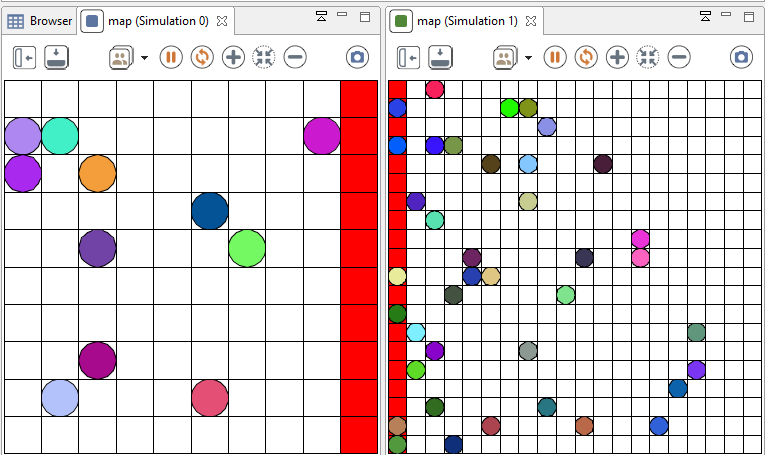
You can also imagine to run two simulations, and to communicate from one to an other through the experiment, as it is shown in this easy model, where agents can move from one simulation to another :

model smallWorld

global {
	int grid_size <- 10;
	bool modelleft <- true;
	int id<- 0;
	int nb_agents <- 50;

	init {
		create people number: nb_agents {
			my_cell <- one_of(cell);
			location <- my_cell.location;
		}
		if (modelleft) {
			ask cell where (each.grid_x = (grid_size - 1))  {
				color <- #red;
			}
		} else {
			ask cell where (each.grid_x = 0)  {
				color <- #red;
			}
		}
	}

	action changeWorld(rgb color, point loc) {
		create people with:[color::color, location::loc] {
			my_cell <- cell(location);
		}
	}
}

species people {
	rgb color <- rnd_color(255);
	cell my_cell;

	reflex move {
		if (modelleft and my_cell.color = #red) {
			ask smallWorld_model[1] {
				do changeWorld(myself.color, {100 - myself.location.x,myself.location.y});
		 	}
		 	do die;
		} else {
			list<cell> free_cells <- list<cell> (my_cell.neighbors) where empty(people inside each);
			if not empty(free_cells) {
				my_cell <- one_of(free_cells);
				location <- my_cell.location;
			}
		}

	}
	aspect default {
		draw circle(50/grid_size) color: color;
	}
}

grid cell width: grid_size height: grid_size;

experiment fromWorldToWorld type: gui {
	init {
		 create simulation with:[grid_size::20, modelleft::false, id::1, nb_agents::0];
	}

	output {
		display map {
			grid cell lines: #black;
			species people;
		}
	}
}
For more complex communication example you can look into the example models from the network plugin>
TCP Server And Client Example .gaml runs a first simulation that will create two servers (one of them being the lead server), then the experiment will create a new simulation with different parameters, and this simulation will itself create two clients, after this, clients and servers from both simulations will communicate together through the TCP protocol. The same behavior can be found in the WebSocket Server And Client Example .gaml model but with the use of websocket instead of TCP.
Going a step further, TCP Teleportation.gaml recreates the same behavior as the Small world example from the previous statement but this time the whole agent is serialized and de-serialized from one simulation to another then sent through TCP. And this time you can chain as many simulation as you want thanks to an experiment parameter. 1 Pong Teleportation (send agent).gaml exhibits the same behavior but uses the MQTT protocol.
Here is an other example of application available in the model library under the name Ant Foraging.gaml with the experiment 3 Simulations. In this simulation, we run 3 times the Ant Foraging model, with different parameters and plot in a unique graph the evolution of the total gathered food by each model.

This graph is done thanks to the permanent block:
permanent {
	display Comparison background: #white {
		chart "Food Gathered" type: series {
			loop s over: simulations {
				data "Food " + int(s) value: s.food_gathered color: s.color marker: false style: line thickness: 5;
			}
		}
	}
}
This block defines a display that is linked to the experiment only, it can thus access all the currently running simulations with the list simulations. From there you can define displays to summarize what's happening in all the simulations, display some statistics on them etc.
If you run several simulations, you may want to use the same seed for each one of those simulations (to compare the influence of a certain parameter, in exactly the same conditions).
Let's remind you that seed is a built-in attribute of the model. You than just need to specify the value of your seed during the creation of the simulation if you want to fix the seed :
create simulation with:[seed::10.0];
You can also specify the seed if you are inside the init scope of your global agent.
global {
	init {
		seed<-10.0;
	}
}
Notice that if you affect the value of your seed built-in directly in the global scope, the affectation of the parameters (for instance specified with the facet with of the statement create), and the "init" will be done after will be done at the end.
The experiment agent also have a built-in attribute seed. The value of this seed is defined in your simulation preferences. The first simulation created is created with the seed value of the experiment.
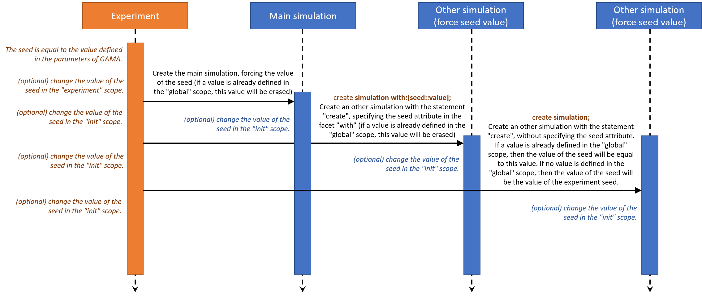
The following sequence diagram can explain you better how the affectation of the seed attribute works :

The affectation of an attribute is always done in this order :
(1) the attribute is affected with a specific value in the species scope. If no attribute value is specified, the value is a default value.
(2) if a value is specified for this attribute in the create statement, then the attribute value is affected again.
(3) the attribute value can be changed again in the init scope.
The following code shows how to run several simulations with a specific seed, determined from the experiment agent :
model multi_simulations

global {
	init {
		create my_species;
	}
}

species my_species skills:[moving] {
	reflex update {
		do wander;
	}
	aspect base {
		draw circle(2) color:#green;
	}
}

experiment my_experiment type:gui  {
	float seedValue <- 10.0;
	float seed <- seedValue; // force the value of the seed.
	init {
		// create a second simulation with the same seed as the main simulation
		create simulation with:[seed::seedValue];
	}
	output {
		display my_display {
			species my_species aspect:base;
		}
	}
}
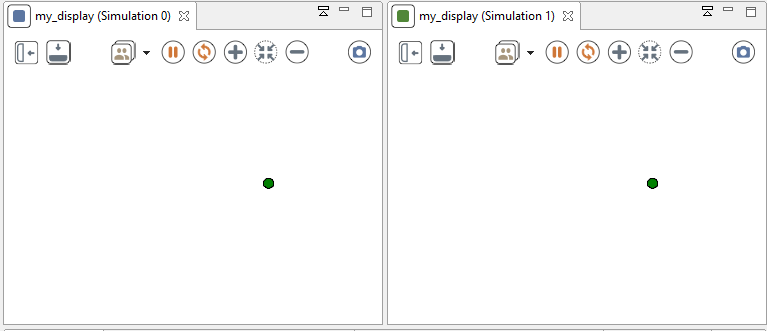
When you run this simulation, their execution is exactly similar.

Let's try now to add a new species in this model, and to add a parameter to the simulation for the number of agents created for this species.
model multi_simulations

global {
	int number_of_speciesB <- 1;
	init {
		create my_speciesA;
		create my_speciesB number:number_of_speciesB;
	}
}

species my_speciesA skills:[moving] {
	reflex update {
		do wander;
	}
	aspect base {
		draw circle(2) color:#green;
	}
}

species my_speciesB skills:[moving] {
	reflex update {
		do wander;
	}
	aspect base {
		draw circle(2) color:#red;
	}
}

experiment my_experiment type:gui  {
	float seedValue <- 10.0;
	float seed <- seedValue; // force the value of the seed.
	init {
		create simulation with:[seed::seedValue,number_of_speciesB::2];
	}
	output {
		display my_display {
			species my_speciesA aspect:base;
			species my_speciesB aspect:base;
		}
	}
}
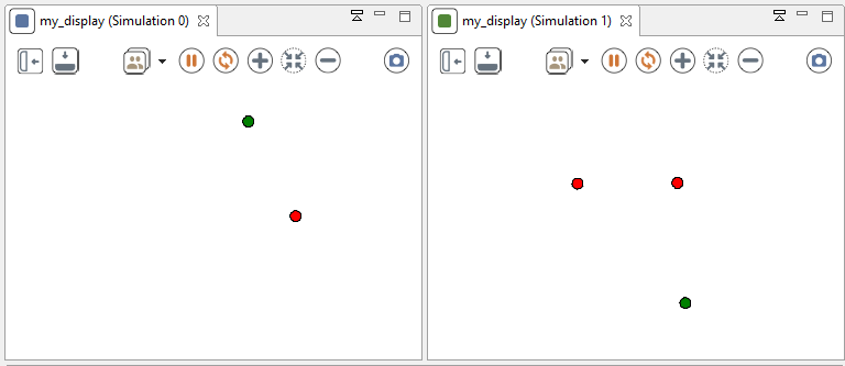
Then you run the experiment, you may find something strange...

Even if the first step seems ok (the green agent and one of the two red agent is initialized with the same location), the simulation differs completely. You should have expected to have the same behavior for the green agent in both of the simulation, but it is not the case. The explanation of this behavior is that a random number generator has generated more random numbers in the second simulation than in the first one.
If you don't understand, here is a short example that may help you to understand better :
model multi_simulations

global {
	int iteration_number <- 1;
	reflex update {
		float value;
		loop times:iteration_number {
			value<-rnd(10.0);
			write value;
		}
		write "cycle "+cycle+" in experiment "+name+" : "+value;
	}
}

experiment my_experiment type:gui  {
	float seedValue <- 10.0;
	float seed <- seedValue; // force the value of the seed.
	init {
		create simulation with:[seed::seedValue,iteration_number::2];
	}
	output {
	}
}
The output will be something like that :
7.67003069780383
cycle 0 in experiment multi_simulations_model0 : 7.67003069780383
7.67003069780383
0.22889843360303863
cycle 0 in experiment multi_simulations_model1 : 0.22889843360303863
0.22889843360303863
cycle 1 in experiment multi_simulations_model0 : 0.22889843360303863
4.5220913306263855
0.8363180333035425
cycle 1 in experiment multi_simulations_model1 : 0.8363180333035425
4.5220913306263855
cycle 2 in experiment multi_simulations_model0 : 4.5220913306263855
5.460148568140819
4.158355846617511
cycle 2 in experiment multi_simulations_model1 : 4.158355846617511
0.8363180333035425
cycle 3 in experiment multi_simulations_model0 : 0.8363180333035425
1.886091659169562
4.371253083874633
cycle 3 in experiment multi_simulations_model1 : 4.371253083874633
Which means :
| Cycle | Value generated in simulation 0 | Value generated in simulation 1 |
|---|---|---|
| 1 | 7.67003069780383 | 7.67003069780383 |
| 0.22889843360303863 | ||
| 2 | 0.22889843360303863 | 4.5220913306263855 |
| 0.8363180333035425 | ||
| 3 | 4.5220913306263855 | 5.460148568140819 |
| 4.158355846617511 |
When writing your models, you have to be aware of this behavior. Remember that each simulation has it's own random number generator.
The RNG (random number generator) can also be changed : rng is a string built-in attribute of the experiment (and also of the model). You can choose among the following rng :
- mersenne (by default)
- parallel
- java
- threaded
The following model shows how to run 4 simulations with the same seed but with some different RNG :
model multi_simulations

global {
	init {
		create my_species number:50;
	}
}

species my_species skills:[moving] {
	reflex update {
		do wander;
	}
	aspect base {
		draw square(2) color:#blue;
	}
}

experiment my_experiment type:gui  {
	float seed <- 10.0;
	init {
		create simulation with:[rng::"threaded",seed::10.0];
		create simulation with:[rng::"java",seed::10.0];
	}
	output {
		display my_display {
			species my_species aspect:base;
			graphics "my_graphic" {
				draw rectangle(35,10) at:{0,0} color:#lightgrey;
				draw rng at:{3,3} font:font("Helvetica", 20 , #plain) color:#black;
			}
		}
	}
}
- Installation and Launching
- Workspace, Projects and Models
- Editing Models
- Running Experiments
- Running Headless
- Preferences
- Troubleshooting
- Introduction
- Manipulate basic Species
- Global Species
- Defining Advanced Species
- Defining GUI Experiment
- Exploring Models
- Optimizing Models
- Multi-Paradigm Modeling
- Manipulate OSM Data
- Cleaning OSM Data
- Diffusion
- Using Database
- Using FIPA ACL
- Using BDI with BEN
- Using Driving Skill
- Manipulate dates
- Manipulate lights
- Using comodel
- Save and restore Simulations
- Using network
- Headless mode
- Using Headless
- Writing Unit Tests
- Ensure model's reproducibility
- Going further with extensions
- Built-in Species
- Built-in Skills
- Built-in Architecture
- Statements
- Data Type
- File Type
- Expressions
- Exhaustive list of GAMA Keywords
- Installing the GIT version
- Developing Extensions
- Introduction to GAMA Java API
- Using GAMA flags
- Creating a release of GAMA
- Documentation generation